In this tutorial we are going to be looking at the SGDR or as referred to in the timm library - the cosine scheduler in little more detail with all the supporting hyperparams.

The SGDR schedule as mentioned in the paper looks like:

from timm.scheduler.cosine_lr import CosineLRScheduler
from nbdev.showdoc import show_doc

class CosineLRScheduler[source]

CosineLRScheduler(optimizer:Optimizer, t_initial:int, lr_min:float=0.0, cycle_mul:float=1.0, cycle_decay:float=1.0, cycle_limit:int=1, warmup_t=0, warmup_lr_init=0, warmup_prefix=False, t_in_epochs=True, noise_range_t=None, noise_pct=0.67, noise_std=1.0, noise_seed=42, k_decay=1.0, initialize=True) :: Scheduler

Cosine decay with restarts. This is described in the paper https://arxiv.org/abs/1608.03983.

Inspiration from https://github.com/allenai/allennlp/blob/master/allennlp/training/learning_rate_schedulers/cosine.py

k-decay option based on k-decay: A New Method For Learning Rate Schedule - https://arxiv.org/abs/2004.05909

The CosineLRScheduler as shown above accepts an optimizer and also some hyperparams which we will look into in detail below. We will first see how we can train models using the cosine LR scheduler by first using timm training docs and then look at how we can use this scheduler as standalone scheduler for our custom training scripts.

Using cosine scheduler with timm training script

To train models using the cosine scheduler we simply update the training script args passed by passing in --sched cosine parameter alongside the necessary hyperparams. In this section we will also look at how each of the hyperparams update the cosine scheduler.

Note: In the paper this scheduler is referred to as SGDR but in timm this is referred to as cosine scheduler. They are both one and the same with minor implementation difference.

The training command to use cosine scheduler looks something like:

python train.py ../imagenette2-320/ --sched cosine

Args

This way we start to use the cosine scheduler with all the defaults. Let's now look at the associated hyperparams and how that updates the annealing schedule.

optimizer

This is the optimizer that will be used for the training process.

from timm import create_model 
from timm.optim import create_optimizer
from types import SimpleNamespace

model = create_model('resnet34')

args = SimpleNamespace()
args.weight_decay = 0
args.lr = 1e-4
args.opt = 'adam' 
args.momentum = 0.9

optimizer = create_optimizer(args, model)

This optimizer object created using create_optimizer is what get's passed to the optimizer argument.

t_initial

The initial number of epochs. Example, 50, 100 etc.

t_mul

Defaults to 1.0. Updates the SGDR schedule annealing.

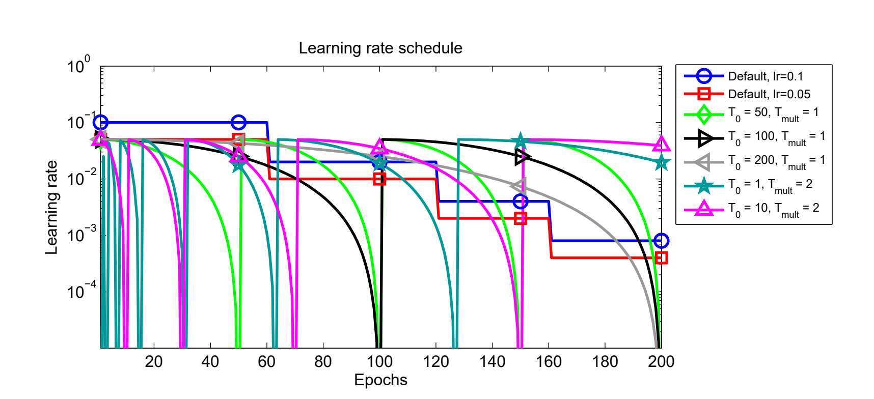
As shown in the image below, here T₀ is the t_initial hyperparameter and T_mult is the t_mul hyperparameter. One can see how updating these parameters updates the scheduler.

lr_min

Defaults to 1e-5. The minimum learning rate to use during the scheduling. The learning rate does not ever go below this value.

decay_rate

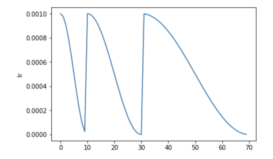
When decay_rate > 0 and <1., at every restart the learning rate is decayed by new learning rate which equals lr * decay_rate. So if decay_rate=0.5, then in that case, the new learning rate becomes half the initial lr.

from matplotlib import pyplot as plt

def get_lr_per_epoch(scheduler, num_epoch):
    lr_per_epoch = []
    for epoch in range(num_epoch):
        lr_per_epoch.append(scheduler.get_epoch_values(epoch))
    return lr_per_epoch

decay_rate=1. or no decay

num_epoch = 50
scheduler = CosineLRScheduler(optimizer, t_initial=num_epoch, decay_rate=1., lr_min=1e-5)
lr_per_epoch = get_lr_per_epoch(scheduler, num_epoch*2)

plt.plot([i for i in range(num_epoch*2)], lr_per_epoch);

decay_rate=0.5

num_epoch = 50
scheduler = CosineLRScheduler(optimizer, t_initial=num_epoch, decay_rate=0.5, lr_min=1e-5)
lr_per_epoch = get_lr_per_epoch(scheduler, num_epoch*2)

plt.plot([i for i in range(num_epoch*2)], lr_per_epoch);

warmup_t

Defines the number of warmup epochs.

warmup_lr_init

The initial learning rate during warmup.

num_epoch = 50
scheduler = CosineLRScheduler(optimizer, t_initial=num_epoch, warmup_t=5, warmup_lr_init=1e-5)
lr_per_epoch = get_lr_per_epoch(scheduler, num_epoch)
plt.plot([i for i in range(num_epoch)], lr_per_epoch, label="With warmup");

num_epoch = 50
scheduler = CosineLRScheduler(optimizer, t_initial=num_epoch)
lr_per_epoch = get_lr_per_epoch(scheduler, num_epoch)
plt.plot([i for i in range(num_epoch)], lr_per_epoch, label="Without warmup", alpha=0.8);

plt.legend();

As we can see by setting up warmup_t and warmup_lr_init, the cosine scheduler first starts with a value of warmup_lr_init, then gradually progresses up to the initial_lr set in the optimizer which is 1e-4. It takes warmup_t number of epochs to go from warmup_lr_init to initial_lr.

warmup_prefix

Defaults to False. If set to True, then every new epoch number equals epoch = epoch - warmup_t.

num_epoch = 50
scheduler = CosineLRScheduler(optimizer, t_initial=num_epoch, warmup_t=5, warmup_lr_init=1e-5)
lr_per_epoch = get_lr_per_epoch(scheduler, num_epoch)
plt.plot([i for i in range(num_epoch)], lr_per_epoch, label="Without warmup_prefix");

num_epoch = 50
scheduler = CosineLRScheduler(optimizer, t_initial=num_epoch, warmup_t=5, warmup_lr_init=1e-5, warmup_prefix=True)
lr_per_epoch = get_lr_per_epoch(scheduler, num_epoch)
plt.plot([i for i in range(num_epoch)], lr_per_epoch, label="With warmup_prefix");

plt.legend();

In the example above we can see how the warmup_prefix updates the LR annealing schedule.

cycle_limit

The number of maximum restarts in SGDR.

cycle_limit=1

num_epoch = 50
scheduler = CosineLRScheduler(optimizer, t_initial=num_epoch, cycle_limit=1)
lr_per_epoch = get_lr_per_epoch(scheduler, num_epoch*2)

plt.plot([i for i in range(num_epoch*2)], lr_per_epoch);

cycle_limit=2

num_epoch = 50
scheduler = CosineLRScheduler(optimizer, t_initial=num_epoch, cycle_limit=2)
lr_per_epoch = get_lr_per_epoch(scheduler, num_epoch*2)

plt.plot([i for i in range(num_epoch*2)], lr_per_epoch);

t_in_epochs

If set to False, the learning rates returned for epoch t are None.

num_epoch = 50
scheduler = CosineLRScheduler(optimizer, t_initial=num_epoch, t_in_epochs=False)
lr_per_epoch = get_lr_per_epoch(scheduler, num_epoch)

lr_per_epoch[:5]

[None, None, None, None, None]

noise_range_t

Add noise to learning rate scheduler.

noise_pct

The amount of noise to be added. Defaults to 0.67.

noise_std

Noise standard deviation. Defaults to 1.0.

noise_seed

Noise seed to use. Defaults to 42.

initialize

If set to True, then, the an attributes initial_lr is set to each param group. Defaults to True.

Note: we leave it up to the reader to try and experiment how the LR annealing scheduling get’s updated by adding in noise hyperparams.